CloudFront Log Collection and Local Visualisation: Seeing What Your Static Site Actually Does
Once the Terraform stack for this blog was running, the obvious next question was: is anyone reading it, and what are they actually requesting? A static site has no application layer to instrument, no request logs on a server you control. Everything flows through CloudFront. So this post covers two things: enabling CloudFront standard logging via Terraform, and building a local Python tool to download, parse, and visualise those logs in the browser.
Update: this post has been revised to reflect a migration from Standard Logging v1 to v2. The original v1 configuration used ACL-based S3 delivery, which stopped working when AWS deprecated that delivery mechanism. The v2 approach uses the CloudWatch Logs Delivery API. The Terraform config, log format, and viewer code have all changed accordingly.
CloudFront Standard Logging
CloudFront has two logging options: standard logging (writes to S3) and real-time logging (streams to Kinesis). For a personal blog, standard logging is the right choice – it captures everything you actually need with minimal operational overhead.
Standard Logging v2 (the current version) delivers log records as gzip-compressed JSON files via the CloudWatch Logs Delivery API. Each file covers a time window of activity at a set of edge locations and lands in S3 within a few minutes of the requests being served. Fields include request time, client IP, URI, status code, bytes served, referrer, user agent, edge location, and more. The delivery is charged as vended logs at $0.50/GB – for a personal blog that is typically a few cents per month.
The earlier Standard Logging v1 used ACL-based delivery and wrote W3C tab-separated files. AWS deprecated that mechanism; this post describes the v2 setup.
The Logs Bucket
The v2 delivery mechanism writes via delivery.logs.amazonaws.com using a bucket policy rather than ACLs, so you don’t need to re-enable ACL support on the bucket. A standard private bucket with a policy allowing the delivery service principal is sufficient:
resource "aws_s3_bucket" "logs" {
  bucket = "${var.domain_name}-logs"
}

resource "aws_s3_bucket_public_access_block" "logs" {
  bucket = aws_s3_bucket.logs.id

  block_public_acls       = true
  block_public_policy     = true
  ignore_public_acls      = true
  restrict_public_buckets = true
}

resource "aws_s3_bucket_policy" "logs" {
  bucket = aws_s3_bucket.logs.id

  policy = jsonencode({
    Version = "2012-10-17"
    Statement = [{
      Sid       = "AllowCloudFrontLogsDelivery"
      Effect    = "Allow"
      Principal = { Service = "delivery.logs.amazonaws.com" }
      Action    = "s3:PutObject"
      Resource  = "${aws_s3_bucket.logs.arn}/*"
      Condition = {
        StringEquals = { "s3:x-amz-acl" = "bucket-owner-full-control" }
      }
    }]
  })
}
The s3:x-amz-acl condition ensures the delivery service sets bucket-owner-full-control on every object it writes, so the objects land in your account with full ownership. Public access remains fully blocked.
Lifecycle Policy
Logs accumulate. A 90-day expiration rule keeps the bucket from growing unboundedly:
resource "aws_s3_bucket_lifecycle_configuration" "logs" {
  bucket = aws_s3_bucket.logs.id

  rule {
    id     = "expire-cloudfront-logs"
    status = "Enabled"

    filter {
      prefix = "AWSLogs/"
    }

    expiration {
      days = 90
    }
  }
}
The prefix filter is AWSLogs/ because that is where v2 delivery actually writes the files – see the next section for why. Scoping the rule by prefix leaves room to store other logs in the same bucket later if needed.
Enabling Logging on the Distribution
Standard Logging v2 is not configured via a block inside aws_cloudfront_distribution. Instead it uses three separate CloudWatch Logs Delivery API resources that are wired together:
resource "aws_cloudwatch_log_delivery_source" "cloudfront" {
  provider     = aws.us_east_1
  name         = "${replace(var.domain_name, ".", "-")}-cloudfront"
  log_type     = "ACCESS_LOGS"
  resource_arn = aws_cloudfront_distribution.blog.arn
}

resource "aws_cloudwatch_log_delivery_destination" "cloudfront_s3" {
  provider      = aws.us_east_1
  name          = "${replace(var.domain_name, ".", "-")}-cloudfront-s3"
  output_format = "json"

  delivery_destination_configuration {
    destination_resource_arn = aws_s3_bucket.logs.arn
  }
}

resource "aws_cloudwatch_log_delivery" "cloudfront" {
  provider                 = aws.us_east_1
  delivery_source_name     = aws_cloudwatch_log_delivery_source.cloudfront.name
  delivery_destination_arn = aws_cloudwatch_log_delivery_destination.cloudfront_s3.arn

  s3_delivery_configuration {
    suffix_path                 = "cloudfront/{yyyy}/{MM}/{dd}/{HH}/"
    enable_hive_compatible_path = false
  }
}
Three constraints to note. First, all three resources must use provider = aws.us_east_1 – the CloudFront ACCESS_LOGS log type is only supported in that region regardless of where the rest of your infrastructure lives, the same constraint that applies to ACM certificates. Second, the resource name fields must match [\w-]* (word characters and hyphens only), so dots in the domain name must be replaced with hyphens; the replace() call handles that.
Third, and the one that actually cost me time: the delivery service automatically prepends AWSLogs/{account-id}/CloudFront/ to whatever suffix_path you configure. So with suffix_path = "cloudfront/{yyyy}/{MM}/{dd}/{HH}/", the real S3 keys end up at AWSLogs/333285332693/CloudFront/cloudfront/{yyyy}/{MM}/{dd}/{HH}/filename.gz. This is not documented prominently and it is easy to miss – the delivery looks healthy in the console while the downloader tooling silently fails to find anything because it was configured to list the wrong prefix. The lifecycle rule prefix in the previous section is AWSLogs/ for the same reason.
After terraform apply, logs start appearing in S3 within a few minutes of traffic hitting the distribution.
The Log Format
Each .gz file contains one JSON object per line (NDJSON). A typical record looks like:
{
  "date": "2026-04-07",
  "time": "01:24:01",
  "x-edge-location": "SYD62-P1",
  "sc-bytes": "4823",
  "c-ip": "203.0.113.42",
  "cs-method": "GET",
  "cs(Host)": "blog.jeakyl.com",
  "cs-uri-stem": "/posts/",
  "sc-status": "200",
  "cs(Referer)": "https://example.com/",
  "cs(User-Agent)": "Mozilla/5.0 ...",
  "x-edge-result-type": "Hit",
  "time-taken": "0.001"
}
Fields with no value are represented as "-" (a JSON string containing a dash). The fields that matter most for a blog are:
| Field | What it tells you |
|---|---|
date, time |
When the request happened |
x-edge-location |
Which CloudFront PoP served it |
sc-bytes |
Bytes sent to the client |
c-ip |
Client IP address |
cs-uri-stem |
Which page was requested |
sc-status |
HTTP status code |
cs(Referer) |
Where the visitor came from |
cs(User-Agent) |
Browser or bot |
x-edge-result-type |
Hit, Miss, or Error – cache performance |
time-taken |
Request latency in seconds |
The Local Visualiser
Rather than ship logs to a SaaS analytics tool, a small self-contained Python script handles everything locally. It lives in logs/ at the repo root and has three jobs: download files from S3, parse them into SQLite, and serve a browser dashboard. Running it without arguments does all three:
source logs/.venv/bin/activate
python logs/view.py
# => Serving at http://127.0.0.1:8765
Or run the steps individually:
python logs/view.py download --since 2026-01-01
python logs/view.py parse
python logs/view.py serve --port 9000
Download
The downloader uses boto3 to paginate list_objects_v2 over the AWSLogs/ prefix (the bucket-scoped prefix CloudFront v2 writes under), then downloads each .gz file to logs/raw/ – skipping any file that already exists locally. Filenames are unique, so filename equality is a reliable cache key.
v2 files land under date-partitioned paths like AWSLogs/{account-id}/CloudFront/cloudfront/2026/04/07/01/filename.gz rather than the flat layout v1 used. The --since flag extracts the date by scanning path segments for a YYYY/MM/DD run, falling back to the filename for old v1 files:
def _date_from_key(key):
    parts = key.split("/")
    # v2: look for a YYYY/MM/DD run anywhere in the path
    for i in range(len(parts) - 2):
        y, m, d = parts[i], parts[i + 1], parts[i + 2]
        if len(y) == 4 and y.isdigit() and len(m) == 2 and m.isdigit() and len(d) == 2 and d.isdigit():
            return f"{y}-{m}-{d}"
    # v1 fallback: find YYYY-MM-DD in the filename
    for segment in parts[-1].split("."):
        chunks = segment.split("-")
        if len(chunks) >= 3:
            candidate = "-".join(chunks[:3])
            try:
                datetime.strptime(candidate, "%Y-%m-%d")
                return candidate
            except ValueError:
                continue
    return None
Scanning for the YYYY/MM/DD run rather than indexing fixed positions means the function keeps working regardless of how many prefix segments the delivery service adds in front. The v1 fallback ensures any existing flat-layout files in logs/raw/ continue to be handled correctly.
Parse
The parser opens each .gz with gzip.open and auto-detects the format from the first content line: if it starts with { the file is v2 JSON, otherwise it falls back to the v1 tab-separated path. This means a logs/raw/ directory containing a mix of old v1 files and new v2 files is handled transparently – no manual intervention needed.
The JSON parser maps CloudFront field names to database columns and applies the same coercion helpers as the v1 path:
_JSON_FIELD_MAP = {
    "c-ip":          ("client_ip",  null_if_dash),
    "cs-uri-stem":   ("uri_stem",   null_if_dash),
    "sc-status":     ("status",     coerce_int),
    "sc-bytes":      ("sc_bytes",   coerce_int),
    "time-taken":    ("time_taken", coerce_float),
    # ... 16 more fields
}
v2-only fields (asn, timestamp(ms), distribution-tenant-id) are ignored. The existing database schema covers all the fields that matter for the dashboard, so no migration is needed when switching from v1 to v2 files.
Rows are bulk-inserted into SQLite via executemany. A second table, ingested_files, tracks which .gz files have been processed so re-running parse is safe and instant when no new files have arrived.
SQLite is a natural fit here. The dataset is small (a personal blog might accumulate a few hundred thousand rows over months), queries are fast, and there are no servers to run. A single data.db file is the entire database.
Serve
The HTTP server is Python’s built-in http.server.HTTPServer with a custom handler. It serves two things:
GET /returnsui.htmlread from disk on every request (no restart needed when editing the dashboard during development).GET /api/<endpoint>runs a parameterised SQLite query and returns JSON.
The API endpoints are:
| Endpoint | Returns |
|---|---|
/api/stats |
Total requests, unique visitors, bytes served, error rate, date range |
/api/timeseries |
Requests per day |
/api/top_pages |
Top 20 URIs by hit count |
/api/status_dist |
Request count grouped by status code |
/api/top_referrers |
Top 15 referrers |
/api/edge_locations |
Hit count per CloudFront PoP |
/api/countries |
Top 30 countries by request count |
/api/search |
Paginated filtered log rows |
All endpoints accept ?start=YYYY-MM-DD&end=YYYY-MM-DD query parameters. All queries use SQLite’s parameterised form – no user input is interpolated into query strings.
The Dashboard
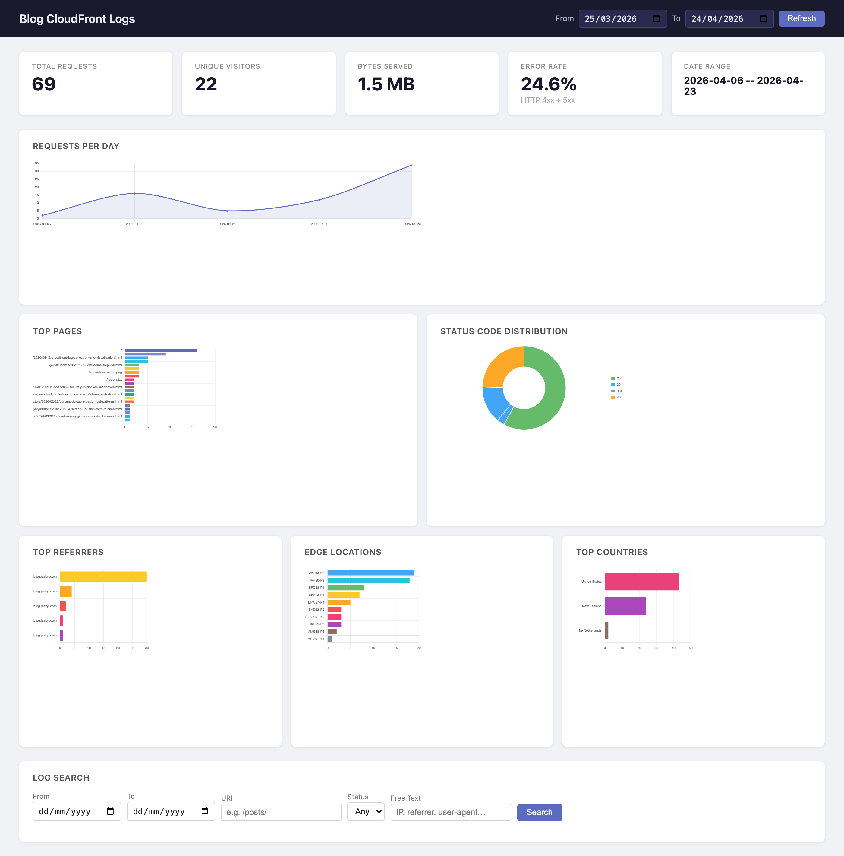
The dashboard is a single ui.html file with no build step and no framework. Chart.js loads from a CDN and the page fetches all data from the local API via fetch() on page load.
The page defaults to the last 30 days on load. A date-range picker in the header and a Refresh button reload all charts for the selected range.
Charts:
- Requests per day – line chart with fill, useful for spotting traffic spikes or drops
- Top pages – horizontal bar, because URI strings are long and read poorly in vertical bars
- Status code distribution – doughnut, showing the proportion of 2xx/3xx/4xx/5xx at a glance
- Top referrers – horizontal bar, hostname extracted from the full URL
- Edge locations – horizontal bar, showing which CloudFront PoPs are active
- Top countries – horizontal bar, populated once GeoIP data has been loaded (see below)
The search section at the bottom lets you filter by date range, URI substring, status code class (2xx, 3xx, 4xx, 5xx, or specific codes), and free text matched against URI, referrer, IP, and user agent. Results include a Country column showing the ISO code with the full name on hover. Results are paginated at 100 rows with next/previous navigation.
GeoIP: Country-Level Breakdowns
CloudFront logs record the client IP on every request. Mapping that to a country requires a GeoIP database. MaxMind’s GeoLite2-Country is free with a registered account – it’s a single ~7 MB .mmdb binary that covers the full IPv4 and IPv6 space.
The visualiser has a geoip subcommand that downloads it:
python logs/view.py geoip --key YOUR_LICENSE_KEY
# or: export MAXMIND_LICENSE_KEY=YOUR_KEY && python logs/view.py geoip
It downloads the tar.gz from MaxMind, extracts just the .mmdb file into logs/geoip/ (gitignored), and exits. The database is updated by MaxMind weekly; re-run the command to refresh it.
Once the database is present, parse enriches rows automatically as they are inserted:
import geoip2.database

with geoip2.database.Reader("logs/geoip/GeoLite2-Country.mmdb") as reader:
    resp = reader.country("203.0.113.42")
    resp.country.iso_code  # "AU"
    resp.country.name      # "Australia"
For rows already in the database from a previous parse run, there is an enrich subcommand that backfills the two new columns:
python logs/view.py enrich
# Enriching 48,203 rows ...
# Done: 47,891 / 48,203 rows enriched with country data.
It reads all rows where country_code IS NULL, looks up each unique IP once (cached in memory for the duration of the run), and bulk-updates in a single transaction.
The schema migration is non-destructive. When ensure_schema runs against an existing database, it checks PRAGMA table_info(requests) and only issues ALTER TABLE ... ADD COLUMN if country_code or country_name are absent. Existing rows and indexes are untouched.
The ~300 rows that don’t enrich are typically private-range IPs (10.x, 172.16.x, 192.168.x) from CloudFront’s internal health checks, or IP addresses that MaxMind doesn’t have coverage for.
What It Actually Shows
The most immediately useful thing is the top pages chart. For a blog, most traffic goes to the home page and a handful of posts. If one post is getting disproportionate traffic, you can see it immediately.
The referrers chart tells you where readers come from. Direct traffic shows as - (no referrer). Search engine traffic usually shows as Google or Bing. RSS readers show their own domains.
The edge locations chart shows the geographic distribution of your audience indirectly. If most hits come from SYD (Sydney), your readers are in Australia. IAD is Northern Virginia, LHR is London, and so on. CloudFront location codes aren’t documented formally, but they follow IATA airport codes.
The countries chart gives you the same picture directly, with full country names. The distinction between edge locations and countries is useful: a reader in New Zealand may hit the SYD edge (closest PoP), so edge location and country don’t always align perfectly.
The status distribution is useful for spotting problems. A healthy blog should be almost entirely 2xx and 3xx (redirects). 4xx spikes usually mean a post URL changed without a redirect in place, or a bot is probing paths. 5xx would indicate something wrong with the build or the S3 bucket.
The x-edge-result-type field (stored as edge_result_type) tells you cache performance. Hit means CloudFront served from cache without hitting S3. Miss means it fetched from the origin. For a static blog with Managed-CachingOptimized, the hit rate should be high after the first few requests to each URL.
What’s Not Here
Standard CloudFront logs have a delay of a few minutes to a few hours. If you need sub-minute latency, that’s what real-time logging to Kinesis is for – but that costs real money and adds operational complexity that isn’t worth it for a personal blog.
The visualiser has no authentication. It binds to 127.0.0.1 by default, so it’s only accessible locally. Don’t expose it on a public interface.
Summary
Enabling CloudFront Standard Logging v2 is four Terraform resources on the infrastructure side: a logs bucket, public access block, bucket policy, and lifecycle rule. Plus three CloudWatch Logs Delivery API resources (source, destination, delivery) that wire the distribution to the bucket. All delivery resources must be in us-east-1. The cost is the S3 storage plus vended log delivery at $0.50/GB – for a personal blog that works out to a few cents per month.
The local visualiser is around 650 lines of Python and 350 lines of HTML/JS, using nothing beyond the stdlib, boto3, and geoip2. SQLite handles the storage. The whole thing runs with one command and opens in the browser. For a personal blog, that’s the right level of complexity – enough to see what’s happening, simple enough to understand and modify.